My first introduction to Pokemon was back when Pokemon Yellow came out, I would watch my cousin play on his Game Boy. It wouldn’t be until many years later when I got my first job that I would finally play my own Pokemon game. It was Pokemon Emerald!, I remember wanting to have all the legendaries (and there were so many in Emerald) since obviously they must have the best stats, but eventually I lost interest in that strategy and just started using meta teams.
But shouldn’t meta teams be all legendaries? It didn’t make sense to have Gardevoir instead of Latias in the team. So if a legendary isn’t always the best in slot, what makes it a legendary? The obvious answer is its rarity, but I wanted to go deeper and see how legendaries compared to regular Pokemon.
If you are not interested in the data analysis process and only want to see the final result, skip to Final Result :).
Since I am just starting my journey on data analysis, I thought this would be good first task. For tools I am keeping it simple and using just Python with the libraries: pandas for loading and processing the data and matplotlib for visualization.
First Look At The Data
For this analysis, I’m using the Pokemon Stats Dataset from Kaggle:
The Pokemon Stats dataset provides a comprehensive analysis of the various attributes and characteristics of Pokemon species in the popular video game franchise. Pokemon is a game where players collect and train fictional creatures called "Pokemon" to battle against other trainers.
This database contains the stat values of all Pokemon from generation 1 to 8 and if it’s a legendary or not.
Initial Exploration
We start off with by adding the basic imports and loading the dataset
import pandas as pd
import matplotlib.pyplot as plt

pokemon_data = pd.read_csv("pokemon.csv")
pokemon_data.info()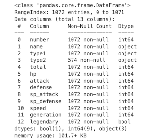
From the info command, we can see that all the base stats are here, as well as the generation and legendary status, which is what we need for our analysis. We can also see that every Pokemon has it’s information as there are no null values, except for type2, but that’s because not all Pokemon have 2 types.
Can we talk about how many Pokemon there are? I played Scarlet and Violet but never stoped to think about there being over 1000 Pokemon already! Crazy!
From this basic info we got, we can see that this dataset is already cleaned, or at least it doesn’t have any null values that we have to deal with. When we get more into it [spoiler] we will find that it includes Pokemon variations we might not want in our analysis such as Ash’s Greninja or the Mega variations. For this specific analysis we will keep these entries.
The Legendary Question
My first question here is, how many of these 1072 Pokemon are legendaries? Let’s check:
pokemon_data.legendary.sum()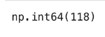
This returns a count of 118 legendary Pokemon. That’s 11% of the total count, I was expecting legendaries to be more rare. Now, we will compare average stats for legendaries and non legendaries.
# Create a comparison chart
stats_to_compare = ['hp', 'attack', 'defense', 'sp_attack', 'sp_defense', 'speed']

legendary_stats = pokemon_data[pokemon_data['legendary'] == True][stats_to_compare].mean()
regular_stats = pokemon_data[pokemon_data['legendary'] == False][stats_to_compare].mean()

# Create side-by-side bar chart
fig, ax = plt.subplots(figsize=(12, 6))
x = range(len(stats_to_compare))
width = 0.35

ax.bar([i - width/2 for i in x], regular_stats, width, label='Regular Pokemon')
ax.bar([i + width/2 for i in x], legendary_stats, width, label='Legendary Pokemon')

# Add value labels on top of bars
for i, v in enumerate(regular_stats):
    ax.text(i - width/2, v + 1, f'{v:.1f}', ha='center', va='bottom')
for i, v in enumerate(legendary_stats):
    ax.text(i + width/2, v + 1, f'{v:.1f}', ha='center', va='bottom')

ax.set_xlabel('Stats')
ax.set_ylabel('Average Value')
ax.set_title('Legendary vs Regular Pokemon: Average Stats')
ax.set_xticks(x)
ax.set_xticklabels(stats_to_compare)
ax.legend()
plt.show()
Here, we calculated the mean values for each stat and plotted them in a comparison bar chart for easier visualization. This is the result.
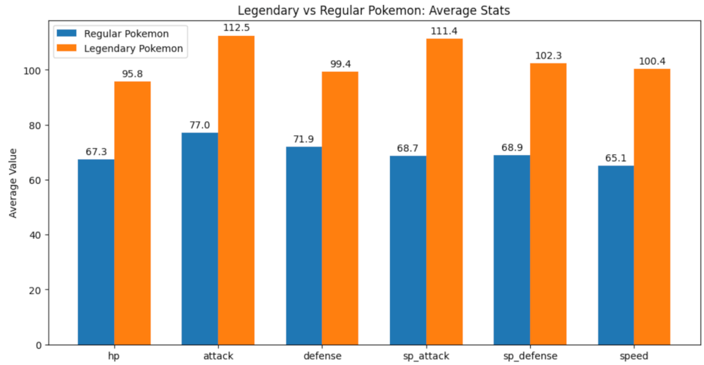
Unsurprisingly, there is a large difference in all of the stats, but let’s consider that we have Pokemon such as Unown and Delibird that have terrible base stats, so they could be affecting the average stats of the Regular Pokemon. These are outliers, and sometimes (if not most) it’s beneficial to exclude them or minimize the impact they could have in our analysis. In this specific analysis, we will use the median operation to replace the mean, this will reduce the impact of outliers.
Kitty Tip!
Outliers are data points that deviate significantly from the typical pattern in your dataset. These data points can throw off your analysis by making averages misleading or making us miss important patterns. Common approaches to handle outliers include removing obvious errors, using robust statistics (like median instead of mean), transforming the data, or analyzing outliers separately to understand what makes them different.
Using the median instead of the mean we get the following chart
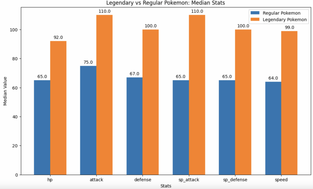
There is a difference, but not as I expected. Instead of the Regular Pokemon catching up to the Legendaries with higher stats, removing outliers actually lowered them more. So our outliers weren’t the Unowns and Delibirds, it was Slaking and the Mega evolutions.
Either way we look at it, Legendary Pokemon as a group have considerably better stats than Regular Pokemon. But now I’m curious about these outliers. Who are the strongest and who are the weakest?
weakest_legendary = pokemon_data[pokemon_data['legendary'] == True].nsmallest(5, 'total')
strongest_legendary = pokemon_data[pokemon_data['legendary'] == True].nlargest(5, 'total')
strongest_regular = pokemon_data[pokemon_data['legendary'] == False].nlargest(5, 'total')

print("Weakest Legendary Pokemon:")
print(weakest_legendary[['name', 'total']])
print("Stringest Legendary Pokemon:")
print(strongest_legendary[['name', 'total']])

print("\nStrongest Regular Pokemon:")
print(strongest_regular[['name', 'total']])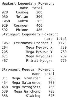
As expected, the Mega evolutions are the ones that skewed the stats. Also, on the weakest Legendary Pokemon, we have mostly pre-evolutions, which also skewed the data. This confirms to me that changing the mean operation with the median was the right choice.
Kitty Tip!
When there are outliers in your data, the mean can be misleading because it gets “pulled” toward those outliers. The median, being the middle value when everything is sorted, is much more stable and often gives you a better sense of what’s “typical” in your dataset.
Digging Deeper
Power Creep
A common occurrence in games that introduce new characters each version or patch, is power creep. This is when new mechanics are introduced where new units have an advantage over old units, or it could be something as simple as the new units being overall stronger than the old ones. To see if this is the case in Pokemon, let’s look at the stats over each generation.
gen_stats = pokemon_data.groupby('generation').agg({
    'total': 'mean',
    'hp': 'mean',
    'attack': 'mean',
    'defense': 'mean',
    'sp_attack': 'mean',
    'sp_defense': 'mean',
    'speed': 'mean',
    'legendary': 'sum'  # Count of legendaries per generation
}).round(2)
fig, (ax1, ax2) = plt.subplots(2, 1, figsize=(12, 10))

# Generation power creep stats
print(gen_stats[['total', 'legendary']].to_string())

print(f"Generation with highest average stats: Gen {gen_stats['total'].idxmax()} ({gen_stats['total'].max():.1f})")
print(f"Generation with lowest average stats: Gen {gen_stats['total'].idxmin()} ({gen_stats['total'].min():.1f})")
print(f"Total stat increase from Gen 1 to latest: {gen_stats['total'].iloc[-1] - gen_stats['total'].iloc[0]:.1f} points")

print(f"\nBiggest stat jump between generations:")
stat_diffs = gen_stats['total'].diff()
biggest_jump = stat_diffs.idxmax()
print(f"Gen {biggest_jump-1} to Gen {biggest_jump}: +{stat_diffs[biggest_jump]:.1f} points")

# Top plot: Average Total Stats by Generation
ax1.plot(gen_stats.index, gen_stats['total'],
         marker='o', linewidth=3, markersize=8, color='#FF6B6B')
ax1.set_title('Pokemon Power Creep: Average Total Stats by Generation',
              fontsize=16, fontweight='bold', pad=20)
ax1.set_xlabel('Generation', fontsize=12)
ax1.set_ylabel('Average Total Stats', fontsize=12)
ax1.grid(True, alpha=0.3)
ax1.set_xticks(gen_stats.index)

for i, v in enumerate(gen_stats['total']):
    ax1.annotate(f'{v:.1f}', (gen_stats.index[i], v),
                textcoords="offset points", xytext=(0,10), ha='center')

# Bottom plot: Individual Stats Breakdown
stats_to_plot = ['hp', 'attack', 'defense', 'sp_attack', 'sp_defense', 'speed']
colors = ['#FF9999', '#66B2FF', '#99FF99', '#FFCC99', '#FF99CC', '#99CCFF']

for stat, color in zip(stats_to_plot, colors):
    ax2.plot(gen_stats.index, gen_stats[stat],
             marker='o', label=stat.replace('_', ' ').title(),
             linewidth=2, markersize=6, color=color)

ax2.set_title('Individual Stat Trends by Generation',
              fontsize=14, fontweight='bold', pad=20)
ax2.set_xlabel('Generation', fontsize=12)
ax2.set_ylabel('Average Stat Value', fontsize=12)
ax2.legend(bbox_to_anchor=(1.05, 1), loc='upper left')
ax2.grid(True, alpha=0.3)
ax2.set_xticks(gen_stats.index)

plt.show()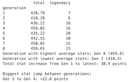
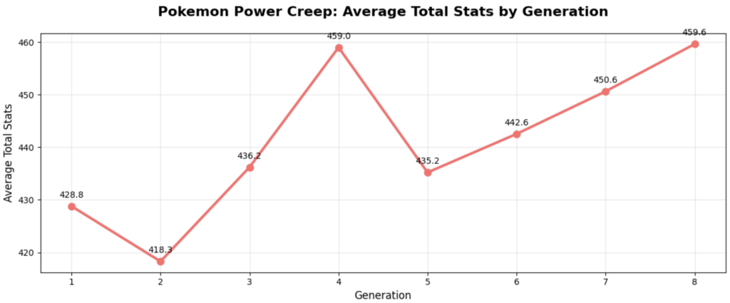
Viewing each generation’s average total stats, we see two dips and one spike. The dip following the 4th generation spike can’t be explained by legendary quantity since generation 5 has a higher legendary count, so this must mean that there are specially powerful Pokemon in the 4th generation. Excluding this, we can see the power creep as the generations progress.
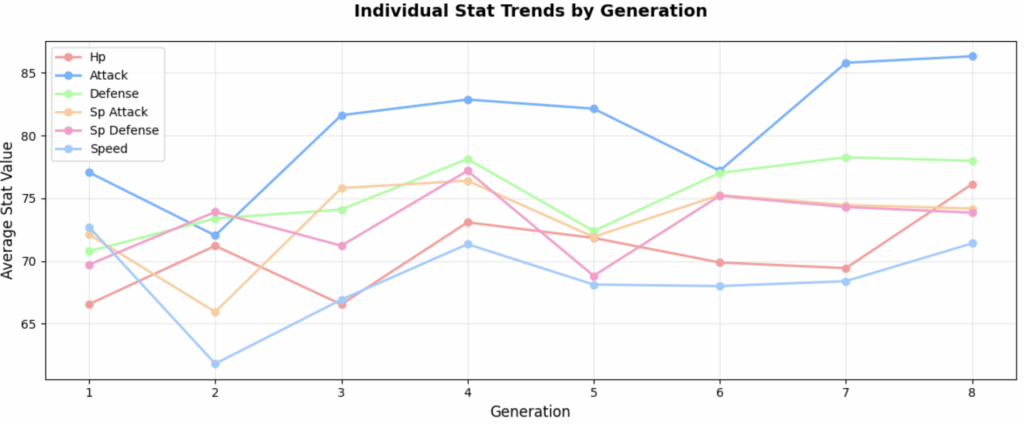
For this one, we can see a few things. First, attack has increased drastically more than defence, we can see the gap between the two growing larger from the first to the eight generation. This can mean that gameplay has gotten more focused on the offensive side in the latest generations.
Also, we can see that Hp has been mostly stable, serving as a balancing anchor as the other stats inflate. This is in contrast to the speed stat, that started with big changes in the first generations, just to be stable in the latest.
If you played all or most of the generations, did you notice these changes? Did you try to use a previous generation team just to notice that they didn’t cut it anymore? Or did you experience the opposite?
Now I want to see if there are any Pokemon with great stats that are not officially legendary. I am picking the total stats cutoff at 618 since that’s the average total stat points for legendaries
pseudo_legendaries = pokemon_data[(pokemon_data['legendary'] == False) & (pokemon_data['total'] >= 618) & (~pokemon_data['name'].str.startswith("Mega"))]
pseudo_legendaries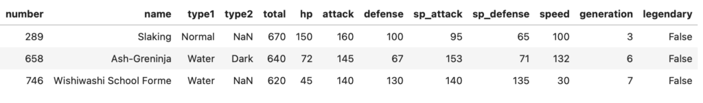
If we don’t count for variations, only Slaking is a pseudo-legendary (according to our definition). He has a crazy attack stat but this gets balanced with his ability that makes him skip every other turn.
Interesting combinations
To finish this up, I wanted to see some interesting stat combinations. Mainly extreme differences in stats of a single Pokemon. Here we will see who has super high attack with super low defence (glass cannons) and the inverse (walls).
glass_cannons = pokemon_data[(pokemon_data['attack'] > 120) & (pokemon_data['defense'] < 60)]
walls = pokemon_data[(pokemon_data['defense'] > 120) & (pokemon_data['attack'] < 60)]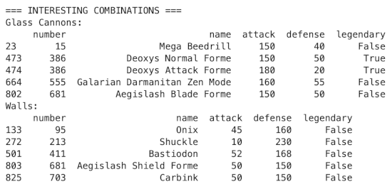
Looking at these stats, and ignoring abilities, moves and types, and only based on raw stats, let’s imagine a battle between Deoxis Attack Forme and Shuckle! Other than the hilarious visuals that would be a very long battle!
What I learned
In conclusion, Legendary Pokemon do have higher stats in general but stats alone don’t make a legendary. We have to consider outliers and how they can affect the criteria we use to classify a Pokemon as legendary.
Mega evolutions, pre evolutions and pseudo legendaries are special cases that prevent us for setting strict thresholds when deciding how to classify a Pokemon. Depending on your goals, there are many ways to deal with this: we can leave everything as it is, we can isolate the special cases and work on the rest of the dataset, or use analysis methods that mitigate the impact of these outliers (such as using median instead of mean like us).
On the side of data analysis, my main lesson when going through this data analysis, is that I have to dedicate more time and energies to the initial data exploration. Just checking for nulls and duplicates is not enough. Some things I missed in the initial exploration: Mega evolutions being included in the dataset and Meltan being in generation 0 (since there is debate on whether it’s from generation 7 or generation 8. Just these two details made me re-adjust the dataset mid-analysis (as can be seen in the notebook).
Finally, this started as an analysis on Legendary Pokemon, but I found other interesting information and ended up being a different analysis from what I planned. And that’s ok, goals aren’t always set in stone.
Final result
Which generation has your favourite Pokemon? Is it keeping up with the current meta? Drop a comment and let me know!
See you next time
Kitty V ^_^
Leave a Reply